Application: Sparse coding / dictionary learning

The dictionary learning / sparse coding problem is defined as follows: there is an unknown \(n\times m\) matrix \(A=(a_1|\cdots|a_m)\) (think of \(m=10n\)). We are given access to many examples of the form \[ y = Ax + e \label{eq:dict-learn} \] for some distribution \(\{ x \}\) over sparse vectors and distribution \(\{ e \}\) over noise vectors with low magnitude.

Our goal is to learn the matrix \(A\), which is called a dictionary.

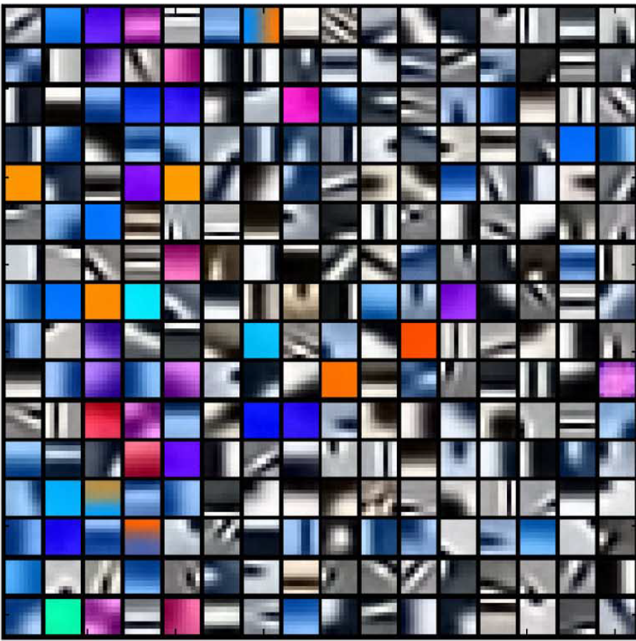
The intuition behind this problem is that natural data elements are sparse when represented in the “right” basis, in which every coordinate corresponds to some meaningful features. For example while natural images are always dense in the pixel basis, they are sparse in other bases such as wavelet bases, where coordinates corresponds to edges etc.. and for this reason these bases are actually much better to work with for image recognition and manipulation. (And the coordinates of such bases are sometimes in a non-linear way to get even more meaningful features that eventually correspond to things such as being a picture of a cat or a picture of my grandmother etc. or at least that’s the theory behind deep neural networks.) While we can simply guess some basis such as the Fourier or Wavelet to work with, it is best to learn the right basis directly from the data. Moreover, it seems that in many cases it is actually better to learn an overcomplete basis: a set of \(m>n\) vectors \(a_1,\ldots,a_m \in \R^n\) so that every example from our data is a sparse linear combination the \(a_k\)’s.Even considering the case that the \(a_m\)’s are a union of two orthonormal bases, such as the standard and Fourier one, already gives rise to many of the representational advantages and computational challenges.

Olshausen and Field (1997) were the first to define this problem - they used a heuristic to learn such a basis for some natural images, and argued that representing images via such an dictionary is somewhat similar to what is done in the human visual cortex. Since then this problem has been used in a great many applications in computational neuroscience, machine learning, computer vision and image processing. Most of the time people use heuristics without rigorous analysis of running time or correctness.

⊕ A dictionary for natural images. This is a set of 256 vectors that offer sparse representation of 8 by 8 pixel patches of natural image. Image taken from Mairal, Elad, and Sapiro (2008)

⊕ Using dictionary learning to remove overlaid text from images. The authors used a dictionary learned from natural images and then removed text from the image by making a “low pass filter” over this dictionary, see Mairal et al. (2009)

There has been some rigorous work using a method known as “Independent Component Analysis” (Comon 1992), but that method makes quite strong assumptions on the distribution \(\{ x \}\) (namely independence). The work of Wang, Wright, and Spielman (2015) has given rise to a different type of rigorously analyzed algorithms based on linear programming, but these all required the vector \(x\) to be very sparse— less than \(\sqrt{n}\) nonzero coordinates. The sos method allows recovery in the much denser case where \(x\) has up to \(\e n\) nonzero coordinates for some \(\e>0\).

From tensor decomposition to dictionary learning

Suppose that \(A=(a_1|\cdots|a_m)\) is a dictionary. For simplicity, we assume that \(\norm{a_i}=1\) for all \(i\), and that the \(a_i\)’s are incoherent in the sense that \(\iprod{a_i,a_j} = o(1)\) for all \(i\neq j\).The assumption on the norm is without loss of generality while some type of incoherence can be shown to be necessary for recovery of the dictionary, regardless of computational issues. Now suppose that we are given many examples \(y_1,\ldots,y_M\) of the form \(y_i = Ax_i+e\) where \(x_1,\ldots,x_M\) are independently sampled from some distribution \(\cD\) over sparse (or nearly sparse) vectors in \(\R^m\) and \(e\) is sampled from a noise distribution with small magnitude. In fact, to simplify things further, for the sake of the current discussion, we will ignore the noise and assume that \(y_i = Ax_i + e\). We will also assume that the distribution on the coefficients \(x\) is symmetric, in the sense that \(\Pr[x]=\Pr[-x]\) and in particular \(\E m(x)=0\) for every square-free monomial \(m\). This is not without loss of generality but is a fairly natural assumption on this disrtribution.

Consider the empirical tensor \(\hat{T} = \tfrac{1}{M} y_i^{\otimes 4}\). If \(M\) is large enough, we can assume that it is essentially the same as the expected tensor \[ T = \E y^{\otimes 4} = \E (Ax)^{\otimes 4} \;. \label{eq:tensor} \]

We will attempt to recover the vectors \(a_1,\ldots,a_m\) by doing a tensor decomposition for \(T\). A priori this might seem like a strange approach since the tensor \(T\) is not going to be proportional to \(\sum_{i=1}^m a_i^{\otimes 4}\). Indeed, by expanding out we can see that this tensor is going to be of the form \[ T = \sum_{i=1}^m (\E x_i^4 ) a_i^{\otimes 4} + O(1)\sum_{1 \leq i,j \leq m} (\E x_i^2 x_j^2) a_i^{\otimes 2}a_j^{\otimes 2} \] where we used the fact that the odd moments of \(x\) vanish.

Now since \(x\) is supposed to be a vector with \(\e m\) nonzero coordinates, let’s consider the simple case where
\(x_i\) is equal to \(\pm 1\) with probability \(\e\) and is equal to \(0\) otherwise and that the distribution is pairwise independent.It can be shown that some bound on the correlation between two coefficients \(x_i\) and \(x_j\) is necessary for recovery. For example, it is a good exercise to show that if \(x_i=x_j\) always then there are two dictionaries \(A,A'\) with distinct set of columns such that the distributions \(y=Ax\) and \(y'=A'x\) are identical. In this case, \(\E x_i^4 = \epsilon\) and \(\E x_i^2x_j^2 = \epsilon^2\).
Now the incoherence assumption implies that the \(n^2\times n^2\) matrix \[ (\sum_i a_i^{\otimes 2})^{\otimes 2} \] will have spectral norm which is \(O(1)\). Hence the tensor \(T\) will have the form \[ T = \epsilon \sum_{i=1}^m a_i^{\otimes 4} + O(\epsilon^2)T' \] where \(T'\) is a \(4\)-tensor that when considered as an \(n^2\times n^2\) matrix has \(O(1)\) spectral norm. Note that the spectral norm of \(\sum_{i=1}^m a_i^{\otimes 4}\) So if \(\epsilon \ll 1\) then what we need is a tensor decomposition algorithm that allows for noise that is small in spectral norm. Note that this is a much stricter condition (in the sense of allowing more noise) than the standard notion of the noise being small when considered as a vector (which corresponds to being small in Frobenius norm). Luckily, the sos based tensor decomposition algorithms can handle this type of noise.

References

Comon, Pierre. 1992. “Independent Component Analysis.” Higher-Order Statistics. Elsevier, 29–38.
Mairal, Julien, Francis Bach, Jean Ponce, and Guillermo Sapiro. 2009. “Online Dictionary Learning for Sparse Coding.” In Proceedings of the 26th Annual International Conference on Machine Learning, 689–96. ACM.
Mairal, Julien, Michael Elad, and Guillermo Sapiro. 2008. “Sparse Representation for Color Image Restoration.” IEEE Trans. Image Process. 17 (1): 53–69. doi:10.1109/TIP.2007.911828.
Olshausen, Bruno A, and David J Field. 1997. “Sparse Coding with an Overcomplete Basis Set: A Strategy Employed by V1?” Vision Research 37 (23). Elsevier: 3311–25.
Wang, Huan, John Wright, and Daniel A. Spielman. 2015. “A Batchwise Monotone Algorithm for Dictionary Learning.” CoRR abs/1502.00064.