The Unique Games and Sum of Squares: A love hate relationship
“Sad to say, but it will be many more years, if ever before we really understand the Mystical Power of Twoness… 2-SAT is easy, 3-SAT is hard, 2-dimensional matching is easy, 3-dimensional matching is hard. Why? of, Why?” Eugene LawlerQuote taken from “The Nature of Computation” by Moore and Mertens.
When computation is involved, very simple objects can sometimes give rise to very complicated phenomena. One of the nicest demonstrations of this is Conway’s Game of Life where a system evolves according to very simple rules, and it has been shown that very simple initial configuration can give rise to highly non trivial patterns.
In the world of efficient computation, one of the simplest and most ubiquitous types of computational problems is the family of constraint satisfaction problems (CSPs). In a CSP instance, one is given a collection of “simple” constraints \(f_1,\ldots,f_m\from\Sigma^n\to\bits\) where \(\Sigma\) is some finite alphabet, often \(\Sigma=\bits\) and the goal is to find an assignment \(x\in\Sigma^n\) so as to maximize the fraction of satisfied constraints \(\tfrac{1}{m}\sum_{i=1}^m f_i(x)\).
Despite seeming simple, the complexity picture of constraint satisfaction problems is not well understood. There are two powerful conjectures whose resolution would significantly clarify this picture: the Feder-Vardi Dichotomy Conjecture (Feder and Vardi 1998) (and its algebraic variant by A. Bulatov, Jeavons, and Krokhin (2005)) for the case of exact computation and Khot’s Unique Games Conjecture (UGC) (Khot 2002) for the case of approximate computation.
We should say that the status of these two conjectures is not identical. The dichotomy conjecture is widely believed and many interesting special cases of it have been proved (in particular for binary and ternary alphabets (Schaefer 1978,Bulatov (2006))). A positive resolution of the dichotomy conjecture would provide a fairly satisfactory resolution of the complexity of exactly computing CSP’s.
In constrat, there is no consensus on the Unique Games Conjecture, and resolving it one way or the other is an extremely interesting open problem. Moreover, as we will see, even a positive resolution of the UGC will not completely settle the complexity of approximating CSP’s, since the existence of an (sos based) subexponential-time algorithm for the Unique Games problem (Arora, Barak, and Steurer 2015) implies that the UGC cannot be used to distinguish between CSP’s who can be approximated in sub exponential time (e.g. \(2^{n^\epsilon}\) for \(1>\epsilon>0\)) and those whose approximation requires exponential time (e.g., \(2^{n^{1-o(1)}}\)).
Defining CSP’s
A CSP is characterized by the family of constraints that are allowed. These constraints are always local in the sense that they only depend on a finite number of coordinates in the input, and then apply one of a family of predicates to these coordinates.
Let \(k\in\N\), \(\Sigma\) be a finite set, and \(\cP\) be a subset of the functions from \(\Sigma^k\) to \(\bits\). The class \(CSP_\Sigma(\cP)\) consists of all instances of the form \(I\) where \(I\) is a subset of \[ \{ f\from\Sigma^n\to\bits \;|\; f(x)= P(x_{i_1},\ldots,x_{i_k}) \text{ for } i_1,\ldots,i_k \in [n] \} \;. \] (When \(\Sigma=\bits\) then we will drop the subscript \(\Sigma\) from \(CSP(\cP)\).)
The value of an instance \(I\in CSP_\Sigma(\cP)\), denoted by \(\val(I)\), is defined as \(\tfrac{1}{|I|}\max_{x\in\Sigma^n} |\{ f\in I : f(x)=1\}|\).
The hypergraph of an instance \(I\), denoted by \(G(I)\) has \(n\) vertices, and \(|I|\) hyperedges, where every hyperedge corresponds to the \(k\) coordinates on which the corresponding constraint depends on.
One example of a CSP is when the family \(\cP\) is generated by applying one or more predicates to the literals in the input which are the variables and their negations in the \(\Sigma=\bits\) case (or their shifts in the larger alphabet case):
Let \(k\in\N\), \(\Sigma\) finite, and \(\cP \subseteq \Sigma^k\to\bits\). We define the family of predicates generated by \(\cP\), denoted as \(\generated{\cP}\), to be the set \[ \{ P\from\Sigma^k\to\bits \;|\; \exists P'\in\cP , \sigma_1,\ldots,\sigma_k \in \Sigma \text{ s.t. } P(x_1,\ldots,x_k)=P'(x_1+\sigma_1,\ldots,x_k+\sigma_k) \} \] where we identify \(\Sigma\) with \(\{0,\ldots,|\Sigma|-1\}\) and addition is done modulo \(|\Sigma|\).
The basic computational problem associated with a CSP is to compute or approximate its value. For simplicity we will be focused on two kinds of decision problems:
- The exact computation problem for \(CSP_\Sigma(\cP)\) is the task of determining, given \(I\in CSP_\Sigma(\cP)\), whether \(\val(I)=1\) or \(\val(I)<1\).
- The \(c\) vs \(s\) approximate computation problem for \(CSP_\Sigma(\cP)\) is the task of distinguishing, given \(I\in CSP_\Sigma(\cP)\), between the case that \(\val(I)\geq c\) and the case that \(\val(I) \leq s\).
Examples:
Here are some classical examples of CSP’s
- \(CSP(\generated{x_1 \vee x_2 \vee \cdots \vee x_k})\) is the \(k-SAT\) problem where one is given a \(k\)-CNF (e.g., \((x_{17} \vee \overline{x}_9 \vee x_{52}) \wedge (\overline{x}_52 \vee x_5 \vee \overline{x}_89)\wedge (x_9 \vee \overline{x}_{22} \vee x_{89})\)) and wants to know if one can satisfy it or, barring that, how close can we get.
- \(CSP(\generated{x_1 \oplus \cdots \oplus x_k})\) is the \(k-XOR\) (also known as \(k\)LIN\((2)\) ) problem.
- If \(\Sigma=\{0,\ldots,k-1\}\) then \(CSP_\Sigma(\{ \neq \})\) is the \(k\) coloring problem. In particular for \(k=2\) this is the Maximum Cut problem
- \(CSP(\{ (x_1 \wedge \cdots \wedge x_{k-1}) \Rightarrow x_k \})\) is known as the HORN sat problem.
- For finite \(\Sigma\) and \(d\in \N\), a \(d\) to \(1\) projection constraint is a predicate \(P\from \Sigma'\times \Sigma \to \bits\) where \(|\Sigma'|=d|\Sigma|\) and where for every \(y\in \Sigma\) there exist exactly \(d\) \(x\)’s in \(\Sigma'\) such that \(P(x,y)=1\). Clearly we can also think of \(P\) as a predicate taking two inputs from the larger alphabet \(\Sigma'\).We can also characterize a \(d\) to \(1\) game as a \(k\) ary predicate \(P\from\Sigma^k\to\bits\) such that \(\Sigma'=P^{-1}(1)\) satisfies that for every \(i\in [k]\) and \(\sigma\in\Sigma\), \(|\{ x\in \Sigma \;|\; x_i = \sigma \}|=d\). The \(d\) to \(1\) problem with alphabet \(\Sigma\) is the CSP corresponding to the set of all \(d\) to \(1\) projection constraints. The \(1\) to \(1\) problem is also known as the unique games problem. The union of the \(d\) to \(1\) problem over all \(d\) is known as the label cover problem.
Classes of CSP’s
At a rough and imprecise level, our intuition from the study of CSP’s is that there are three “canonical prototypes” of CSP problems:
- Linear predicates: These are CSP’s such as \(k\)-XOR where the class of predicates admits some linear or other algebraic structure to allows a Gaussian elimination type algorithm to solve their exact version. The general notion is quite subtle and involves the notion of a polymorphism of the predicate. (Indeed, the technical content of the algebraic dichotomy conjecture is that every predicate admitting such a polymorphism can be solved by a Gaussian elimination type algorithm.)
- Propagation predicates: These are CSP’s such as 2-SAT, Horn-SAT, and Max-Cut where “guessing” few coordinates of the assignment allows us to propagate values for the other coordinates. In particular there is a simple linear time algorithm to solve the exact satisfiability problem of such CSP’s.
- Hard predicates: These are CSP’s such as \(3\)-SAT or \(3\)-COL (as well as their versions with larger arity) where neither an algebraic nor propagation structure is present.
The algebraic dichotomy conjecture can be phrased as the conjecture that the exact decision problem for linear predicates can be solved with a \(poly(n)\) (in fact with exponent at most \(3\)) time algorithm, propagation predicates can be solved with a linear time algorithm, while the exact decision problem for all other predicates is NP hard. In fact, the reduction showing NP hardness for the latter case only has a linear blowup from the 3SAT problem and so, under the exponential time hypothesis, it rules out \(2^{o(n)}\) time algorithms for the exact decision problem for these predicates. The latter two parts (propagation based algorithm and NP hardness reduction) of the dichotomy conjecture have already been proven, and it is the first part that is yet open. To some extent this is not surprising: the Gaussian elimination algorithm is a canonical example of an algorithm using non trivial algebraic structure (and in particular, one that is not captured by the sos algorithm) and understanding its power is a subtle question.
Approximating CSP’s
Considering the notion of approximation of CSP’s makes understanding their complexity harder in some respects and easier in others. Let us focus on the \(1-\epsilon\) vs \(f(\epsilon)\) approximation problem for small \(\epsilon>0\). One aspect in which approximation makes classification easier is that the Gaussian elimination type algorithm are extremely brittle and so the linear predicates actually become hard under noise. This is epitomized by the following theorem of Håstad (2001):
For every \(\epsilon>0\), the \(1-\epsilon\) vs \(1/2+\epsilon\) approximation problem for 3XOR is NP hard.
Moshkovitz and Raz (2010) improved this to give a \(\tilde{O}(n)\) blowup reduction, as well as showing that \(\epsilon\) can tend to zero as fast \(1/polylog(n)\). As far as we know, the fastest algorithm in this problem might require time \(\exp(poly(\epsilon) n)\).
We note that the “brittleness” of Gaussian elimination under noise is also crucially used in cryptography where Lattice based cryptosystems all require for their security the conjecture that solving noisy linear equations is hard, c.f. (Regev 2005) (and in fact for levels of noise that are below those where we can expect to get NP hardness, c.f. (Aharonov and Regev 2004)).
In contrast, the propagation predicates do have non trivial approximation of the form \(1-\epsilon\) vs \(1-f(\epsilon)\) for \(f\) that tends to \(0\) as \(\epsilon\rightarrow 0\). However, understanding the shape of this function \(f(\cdot)\) is an open question, and is to a large extent the content of the Unique Games conjecture. For example, for the Max-Cut problem, the Goemans and Williamson (1995) algorithm yields a \(1-\epsilon\) vs \(1-C\sqrt{\epsilon}\) approximation (for some absolute constant \(C\)) while the best known NP hardness by Trevisan et al. (2000) (which uses a gadget that was found via a computer search) rules out a \(1-\epsilon\) vs \(1-C'\epsilon\) approximation for some absolute \(C'\). Khot et al. (2004) and Mossel, O’Donnell, and Oleszkiewicz (2010) showed that if the Unique Games Conjecture is true, then there is no polynomial-time algorithm beating the guarantee of the Goemans and Williamson (1995) algorithm.
The UGC itself can be phrased as follows:
Unique Games Conjecture: For every \(\epsilon>0\) and \(\delta>0\) there is some \(\Sigma\) such that the \(1-\epsilon\) vs \(\delta\) problem for unique games on alphabet \(\Sigma\) is NP hard.
Give a polynomial-time algorithm that finds a perfectly satisfying solution for a unique game instance if one exists.
Give a polynomial-time algorithm that distinguishes between the case that a unique game instance on \(n\) variables has a \(1-1/(100\log n)\) satisfying solution and the case that every solution satisfies at most \(1/2\) fraction of the instances.Hint: Start by showing this for the case that the graph has bounded maximum degree. Then show that one can assume without loss of generality that the degree is at most a constant when shooting for a \(1/2\) satisfying solution.
While the UGC itself is a constraint satisfaction problem, it has been shown to imply interesting results for other problems as well. Nonetheless, CSP’s provide a very useful lens under which to examine the results and open questions surrounding the UGC.
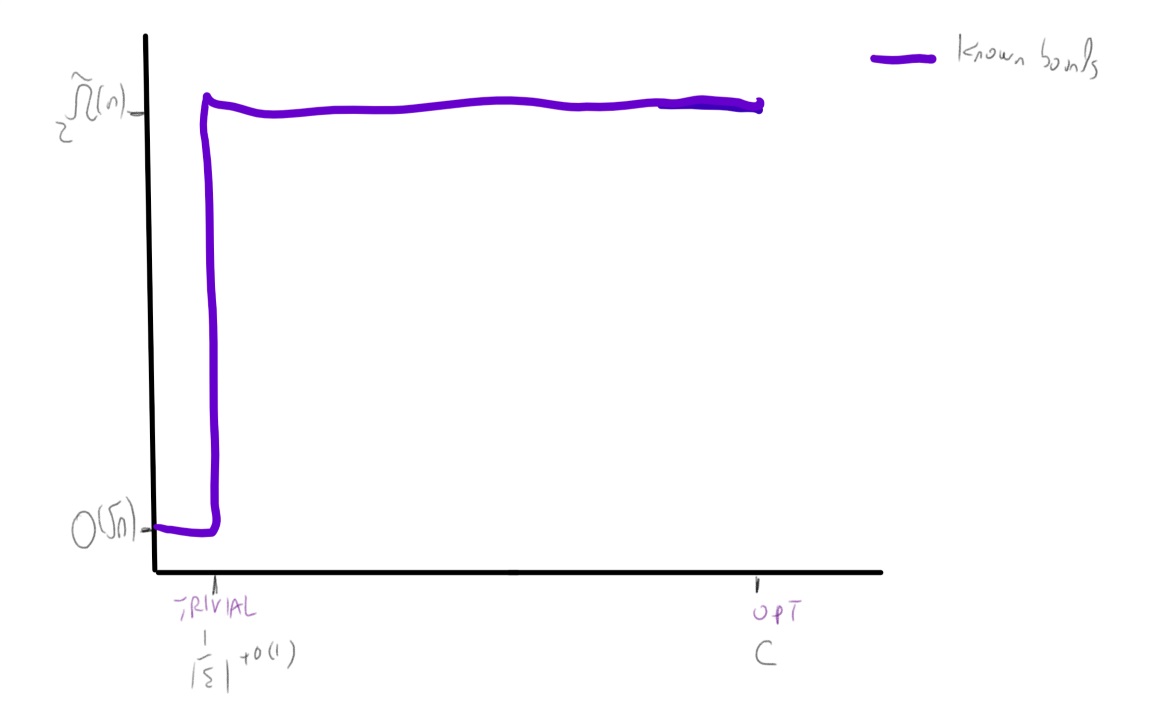
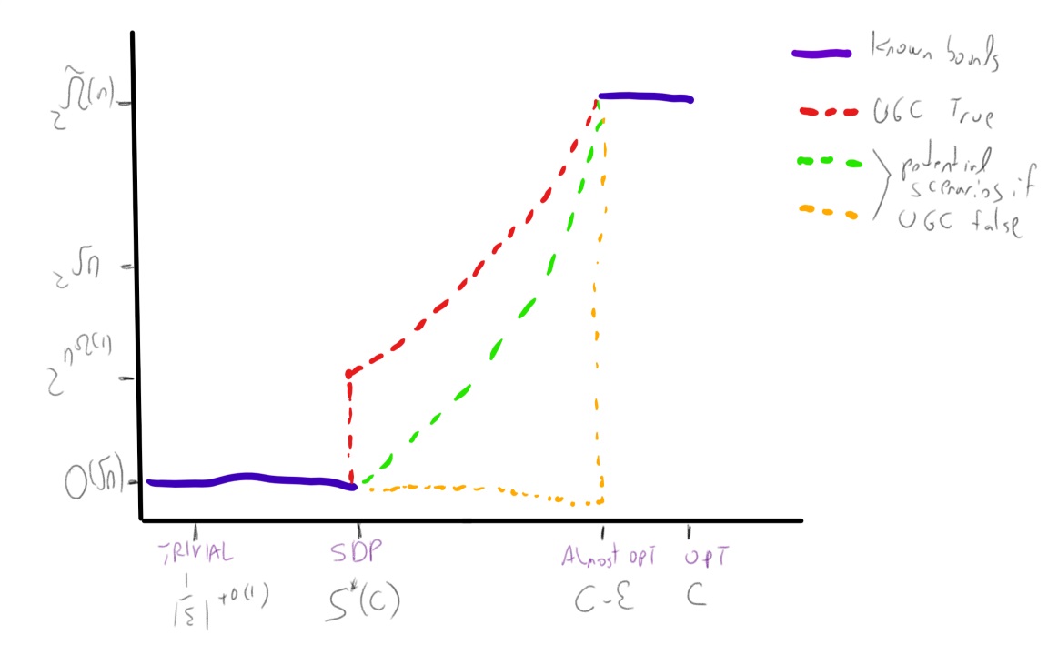
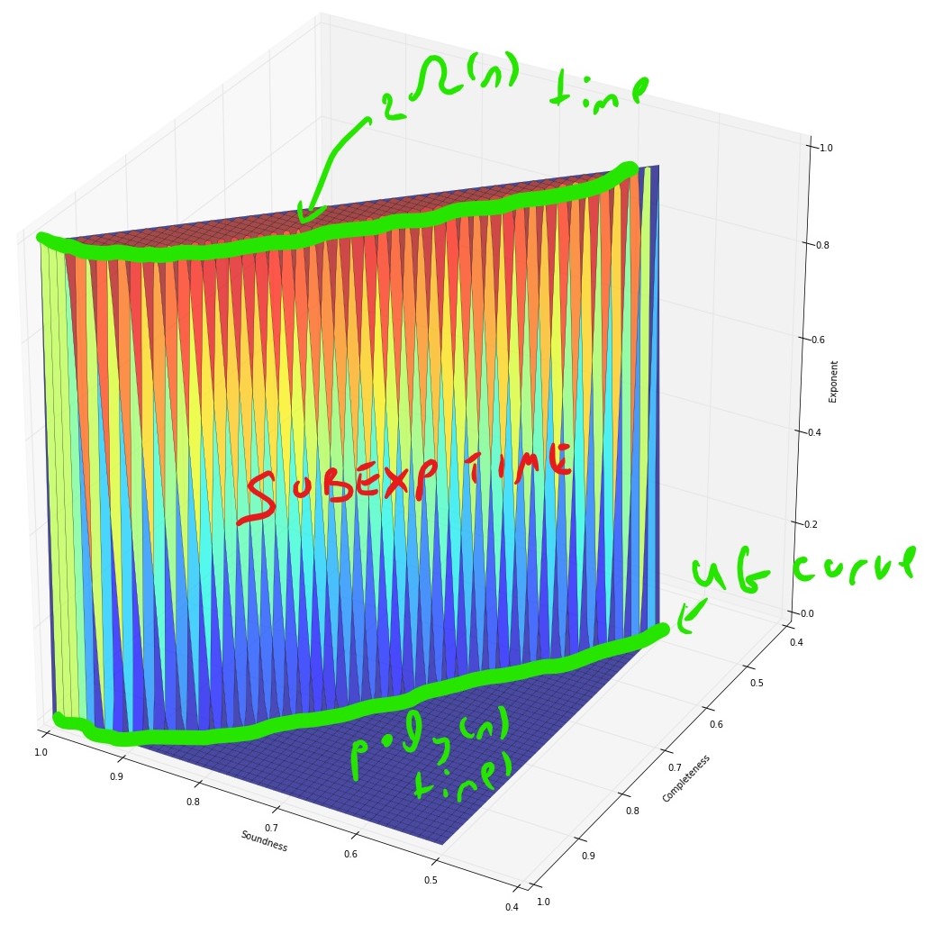
Illustration of the conjectural complexity of CSP’s
If we assume the exponential time hypothesis (Impagliazzo, Paturi, and Zane 1998) and the algebraic dychotomy conjecture (Andrei A. Bulatov, Jeavons, and Krokhin 2005) (both of which are widely believed, especially if we do not distinguish between \(\exp(\Omega(n))\) and \(\exp(n^{1-o(1)})\) running time) then for every exact constraint satisfaction problem can either be solved in \(poly(n)\) (in fact \(O(n^3)\)) time or requires \(\exp(\Omega(n))\) time. The unique games conjecture, coupled with the sub-exponential time algorithm Arora, Barak, and Steurer (2015) shows that the picture for approximation problems is very different. For some CSP’s, such as the “hard” or “linear” CSP’s that contain a pairwise independent distribution, there is a threshold effect similar to the case of exact solution and (up to some measure zero sets) for every two numbers \(0\leq s<c \leq 1\) the task of coming up can either be solved in \(poly(n)\) and or requires \(\exp(n^{1-o(1)})\) time. For others, such as the unique games problem itself (and likely others, such as max cut) there is a region of parameters where the problem can be solved in subexponential time.
Algorithmic results known about the unique games problem.
We denote the unique games problem on alphabet \(\Sigma\) as \(\Sigma\)-UG for short. The following algorithmic results are known about it:
- The basic SDP algorithm (which is a generalization of the Goemans and Williamson (1995) max cut algorithm) can solve the \(1-\epsilon\) vs \(1-O(\sqrt{\epsilon \log |\Sigma|})\) algorithm for the \(\Sigma\)-UG problem, as well as the \(1-\epsilon\) vs \(\Omega(|\Sigma|^{-\epsilon/(2-\epsilon))}\) version of this problem (Charikar, Makarychev, and Makarychev 2006). In particular this means that the \(\Sigma\)-UG problem is not approximation resistant in the sense that there is an algorithm for the \(1-o(1)\) vs \(\tfrac{1}{|\Sigma|}+o(1)\) variant of this problem. It also means that the order of quantifiers in the UGC formulation is crucial, and (unlike the case of 3XOR) we cannot have hardness if the completeness condition holds with parameter \(1-\epsilon\) for \(\epsilon\) tending to zero independently of the alphabet size.
- When \(|\Sigma| \gg 1/\epsilon\) (in particular \(|\Sigma| = 2^{\Omega(1/\epsilon)}\)) then no polynomial time algorithm is known. However, Arora, Barak, and Steurer (2015) showed a \(\exp(\poly(|\Sigma|)n^{\poly(\epsilon)})\) time algorithm for the \(1-\epsilon\) vs \(1/2\) \(\Sigma\)-UG problem.
The approximation guarantees of the Basic SDP algorithm are known to be optimal for \(\Sigma\)-UG if the unique games conjecture is true (Charikar, Makarychev, and Makarychev 2006).
The relation of UGC and the sum of squares algorithm
The UGC and sum of squares algorithm seem to have a sort of “love hate relationship”. For starters, one of the most striking predictions of the UGC is the result of Raghavendra (2008) that if the UGC is true than sos is optimal for all constraint satisfaction problems:
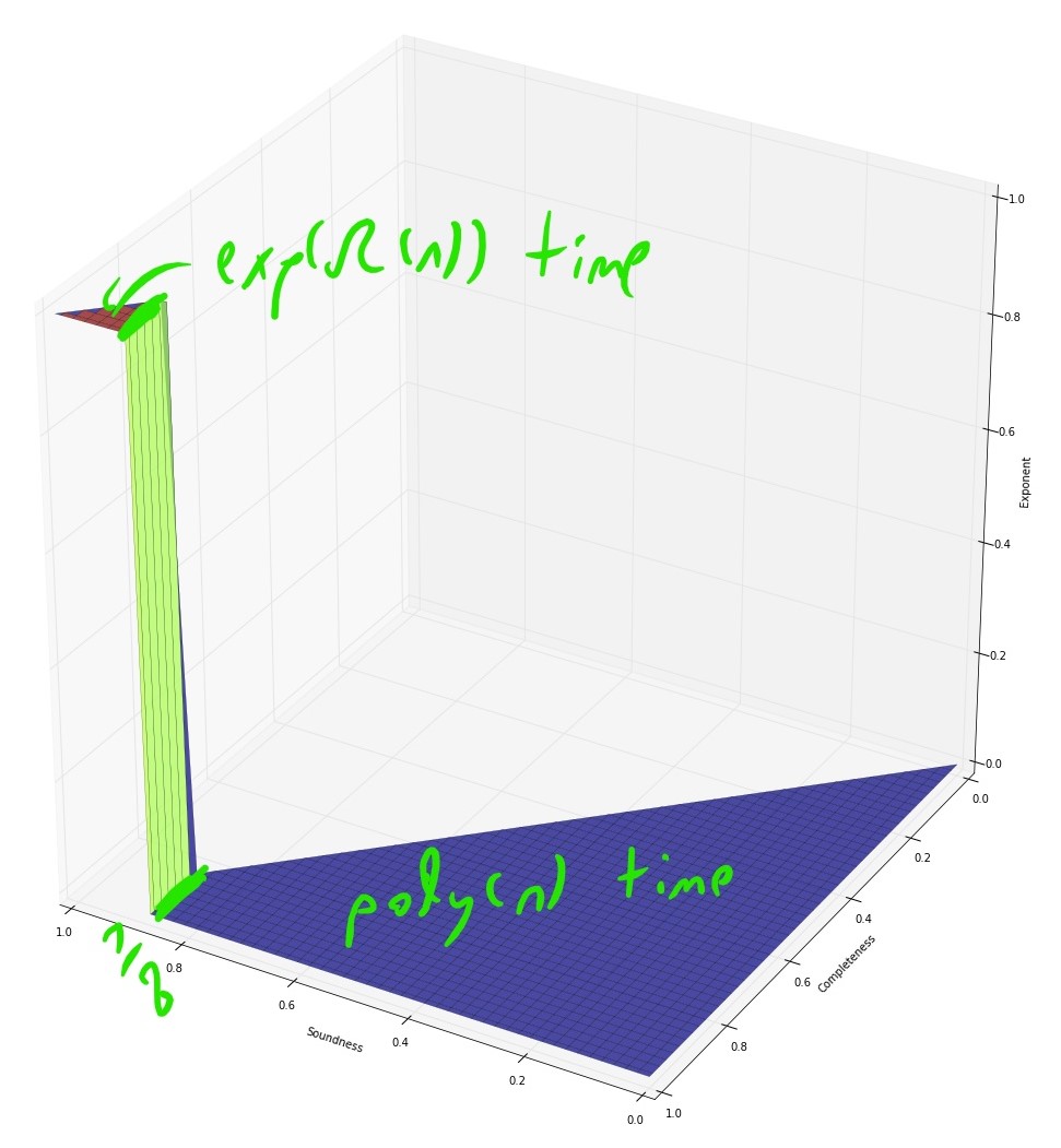
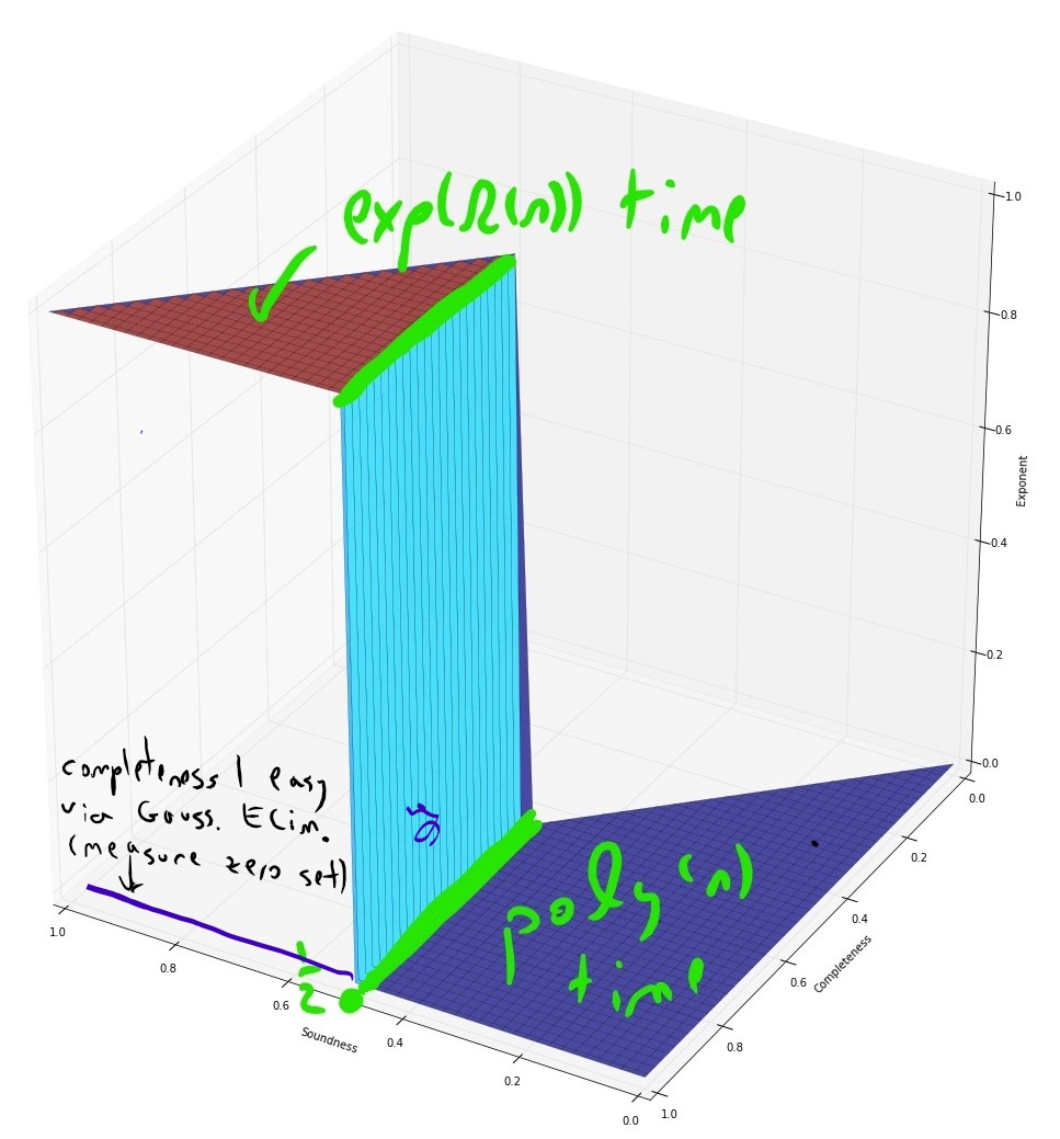
For every \(d\in\N\) and CSP class \(\cC\), define \(f_d(\epsilon)\) to be the infimum over \(n\) going to infinity, of \(\val(I)\) over \(\cC\) instances \(I\) of \(n\) variables such that there is a degree \(d\) pseudo-distribution \(\mu\) such that \(\pE_\mu \val(I) \geq 1-\epsilon\). Then, if the UGC is true then for every CSP class \(\cC\) with arity \(k\), every \(\epsilon>0\), and every \(\delta>0\), the \(1-\epsilon-\delta\) vs \(f_{2k}(\epsilon)\) approximation problem for \(\cC\) is NP hard.
In fact Raghavendra (2008) showed that this holds for a restricted class of pseudo-distributions where the most interesting constraint (namely that \(\pE_\mu p^2 \geq 0\) for all degree \(d/2\) polynomials) needs to hold only for \(d=2\). (These corresponds to solutions of what is known as the “Basic SDP program” for \(\cC\).) Thus the UGC is a “friend” of the sos algorithm in the sense that it shows that it is optimal for a broad class of optimization problems. (Even if it shows that for this class, we don’t really need to use some of the more interesting constraints of the sos algorithm.)
However, the sos algorithm hasn’t always been a friend of the UGC. Arguably the best evidence for the UGC comes from candidate hard instances, which are instances of the unique games problem (or other CSP’s or computational problems) for which the predictions of the UGC hold true for some natural algorithms. That is, the performance of these algorithm is not better than the performance that the UGC predicts is the best possible for polynomial time algorithms. However, the sos algorithm has been used to give some results that call the UGC into questions:
- For the Unique Games problem itself, the sos algorithm gives an \(\exp(n^{poly(\epsilon)})\) time algorithm for the \(1-\epsilon\) vs \(1/2\) unique games problem which is predicted to be NP hard via the UGC. This means that even if the UGC is true, reductions based on it cannot rule out, say, a \(\exp(\sqrt{n})\) time algorithm for any problem. This can also be extended to a \(\exp(n^{\poly(\epsilon)})\) time algorithm for the \(c\) vs \(\epsilon\) \(d\)-to-\(1\) games problem for every absolute constans \(c>0,d\in\N\) that are independent of \(\epsilon\).
- The known hard instances that match the UGC’s predictions are integrality gaps for the Basic SDP program that are CSP instances where for some \(1 \geq c > s \geq 0\), the SDP value is at least \(c\) but it can be proven using various isoperimetric, invariance and concentration results that the true value is at most \(s\). It turns out that the proofs of (sufficiently close variants of) these results can be captured in the constant degree sos proof system, and so there is some constant \(d\) such that the degree \(d\) sos value for these instances is also at most \(s\).
- The unique games conjecture is closely related to a conjecture known as the small set expansion hypothesis (the relation is roughly related to the relation between the Max Cut and Sparsest Cut problems). This latter conjecture is in turn related to the task of finding an (approximately) sparse vector inside a linear subspace, where the sos algorithm does provide non trivial average-case guarantees. It is also related to the Best Separable State problem in quantum information theory, for which the sos algorithm provides non trivial worst case guarantees, though in incomparable parameter regimes. Thus there is a plausible path to refuting the small set expansion hypothesis (and possibly the UGC itself) via sos-based algorithm for finding sparse vectors in a subspace.
Nevertheless, at the moment the status of the UGC is wide open, and indeed some of the efforts to prove the UGC (Khot and Moshkovitz 2016),(Khot, Minzer, and Safra 2016) have also focused on coming up with integrality gaps for the sos program and/or using tools such as the short code (Barak et al. 2012) that have been developed in this context. So, regardless of the final outcome, the sos algorithm and the unique games conjecture will shed a lot of light on one another.
References
Aharonov, Dorit, and Oded Regev. 2004. “Lattice Problems in NP Cap CoNP.” In FOCS, 362–71. IEEE Computer Society.
Arora, Sanjeev, Boaz Barak, and David Steurer. 2015. “Subexponential Algorithms for Unique Games and Related Problems.” J. ACM 62 (5): 42:1–42:25.
Barak, Boaz, Siu On Chan, and Pravesh K. Kothari. 2015. “Sum of Squares Lower Bounds from Pairwise Independence.” In STOC, 97–106. ACM.
Barak, Boaz, Parikshit Gopalan, Johan Håstad, Raghu Meka, Prasad Raghavendra, and David Steurer. 2012. “Making the Long Code Shorter.” In FOCS, 370–79. IEEE Computer Society.
Bulatov, Andrei A. 2006. “A Dichotomy Theorem for Constraint Satisfaction Problems on a 3-Element Set.” Journal of the ACM (JACM) 53 (1). ACM: 66–120.
Bulatov, Andrei A., Peter Jeavons, and Andrei A. Krokhin. 2005. “Classifying the Complexity of Constraints Using Finite Algebras.” SIAM J. Comput. 34 (3): 720–42.
Bulatov, Andrei, Peter Jeavons, and Andrei Krokhin. 2005. “Classifying the Complexity of Constraints Using Finite Algebras.” SIAM Journal on Computing 34 (3). SIAM: 720–42.
Chan, Siu On. 2016. “Approximation Resistance from Pairwise-Independent Subgroups.” J. ACM 63 (3): 27:1–27:32.
Charikar, Moses, Konstantin Makarychev, and Yury Makarychev. 2006. “Near-Optimal Algorithms for Unique Games.” In STOC, 205–14. ACM.
Feder, Tomás, and Moshe Y Vardi. 1998. “The Computational Structure of Monotone Monadic Snp and Constraint Satisfaction: A Study Through Datalog and Group Theory.” SIAM Journal on Computing 28 (1). SIAM: 57–104.
Goemans, Michel X., and David P. Williamson. 1995. “Improved Approximation Algorithms for Maximum Cut and Satisfiability Problems Using Semidefinite Programming.” J. ACM 42 (6): 1115–45.
Håstad, Johan. 2001. “Some Optimal Inapproximability Results.” J. ACM 48 (4): 798–859.
Impagliazzo, Russell, Ramamohan Paturi, and Francis Zane. 1998. “Which Problems Have Strongly Exponential Complexity?” In FOCS, 653–63. IEEE Computer Society.
Khot, Subhash. 2002. “On the Power of Unique 2-Prover 1-Round Games.” In Proceedings of the Thirty-Fourth Annual ACM Symposium on Theory of Computing, 767–75. ACM, New York. doi:10.1145/509907.510017.
Khot, Subhash, and Dana Moshkovitz. 2016. “Candidate Hard Unique Game.” In STOC, 63–76. ACM.
Khot, Subhash, Guy Kindler, Elchanan Mossel, and Ryan O’Donnell. 2004. “Optimal Inapproximability Results for Max-Cut and Other 2-Variable Csps?” In FOCS, 146–54. IEEE Computer Society.
Khot, Subhash, Dor Minzer, and Muli Safra. 2016. “On Independent Sets, 2-to-2 Games and Grassmann Graphs.” Electronic Colloquium on Computational Complexity (ECCC) 23: 124.
Moshkovitz, Dana, and Ran Raz. 2010. “Sub-Constant Error Probabilistically Checkable Proof of Almost-Linear Size.” Computational Complexity 19 (3): 367–422.
Mossel, Elchanan, Ryan O’Donnell, and Krzysztof Oleszkiewicz. 2010. “Noise Stability of Functions with Low Influences: Invariance and Optimality.” Annals of Mathematics. JSTOR, 295–341.
O’Donnell, Ryan, and Yi Wu. 2008. “An Optimal Sdp Algorithm for Max-Cut, and Equally Optimal Long Code Tests.” In STOC, 335–44. ACM.
Raghavendra, Prasad. 2008. “Optimal Algorithms and Inapproximability Results for Every Csp?” In STOC, 245–54. ACM.
Regev, Oded. 2005. “On Lattices, Learning with Errors, Random Linear Codes, and Cryptography.” In STOC, 84–93. ACM.
Schaefer, Thomas J. 1978. “The Complexity of Satisfiability Problems.” In Proceedings of the Tenth Annual Acm Symposium on Theory of Computing, 216–26. ACM.
Trevisan, Luca, Gregory B. Sorkin, Madhu Sudan, and David P. Williamson. 2000. “Gadgets, Approximation, and Linear Programming.” SIAM J. Comput. 29 (6): 2074–97.