Limitations of the sum of squares algorithm
In the last lecture we have seen how the sum of squares algorithm can achieve non-trivial performance guarantees for several interesting problems. But it is not all powerful. In this lecture we will see some negative results for the sum of squares algorithm, showing lower bounds on the degree needed to certify certain problems. In many cases, we do not know of any algorithms that do better, but in some cases we do, and we will see examples of both types. In the standard parlance, these negative results are known as integrality gaps, since these are instances in which there is a gap between the value that the pseudo-distribution “pretends” and the true objective value.The name “integrality gap”, as well as the related notion of a “rounding algorithm” arise from the setting of using a linear program as a relaxation of an integer linear program, where the optimal value of the linear programming relaxation is known as the fractional value, and the opitmal value of the integer linear program is known as the integral value.
The cycle as an integrality gap for Cheeger’s Inequality and Max-Cut
Recall that the discrete Cheeger’s inequality states that every \(d\)-regular graph \(G\) with adjacency matrix \(A\) satisfies \(\lambda \geq \Omega(\varphi(G)^2)\), where \(\lambda\) is the second smallest eigenvalue of the normalized Laplacian \(L_G = I - \tfrac{1}{d}A\). It turns out the humble cycle shows that this bound is tight.
Let \(C_n\) be the cycle on \(n\) vertices and let \(L_{C_n}\) be its normalized Laplacian. Then the second smallest eigenvalue of \(L_{C_n}\) is at most \(O(1/n^2)\).
The lemma shows that Cheeger’s inequality is tight for the \(C_n\) because every subset \(S\subseteq V(C_n)\) with \(1\le \card{S}\le n-1\) has at least one neighbor outside of \(S\). Therefore, the expansion of \(C_n\) is at least \(\varphi(C_n) \geq \Omega(1/n)\).
Let \(\omega=e^{2\pi {\mathrm{i}}/n}\in {\mathbb C}\) be the \(n\)-th root of unity. The vector \(v = (\omega^0,\omega^1,\dots,\omega^{n-1})\) is orthogonal to the all-ones vector \(\Ind\), \[ \iprod{v,\Ind} = \sum_{\ell=0}^{n-1} \omega^\ell = \frac {\omega^0 - \omega^n}{1- \omega} = 0 \] using the formula for the sum of a geometric progression. At the same time, we can upper bound the quadratic form of \(L_{C_n}\) at \(v\), \[ \begin{aligned} \iprod{v,L_{C_n} v} & = \sum_{\ell=0}^{n-1} \abs{\omega^\ell - \omega^{\ell+1}}^2 \\ & = \abs{1-\omega}^2 \cdot n\\ & \le O(1/n^2)\cdot \norm{v}^2\,. \quad \text{} \end{aligned} \] The last step uses \(|1-\omega|^2= O(1/n^2)\). It follows that the second smallest eigenvalue of \(L_{C_n}\) is \(O(1/n^2)\)In fact, it turns out that the second eigenvalue of \(L_{C_n}\) is exactly \(\iprod{v,L_{C_n} v} / \norm{v}^2\) and \(v\) is an eigenvector corresponding to this eigenvalue.
In one of the exercises in the chapter about Max Cut you showed that if a graph \(G\) satisfies \({\mathrm{maxcut}}(G) \leq 1 -\e\) then every degree-\(2\) pseudo-distribution \(\mu\) satisfies that \(\pE_\mu f_G(x) \leq 1 - \Omega(\e^2)\). The following lemma shows that this tradeoff is tight for cycles with an odd number of vertices. Concretely, if \(n\) is odd then \(C_n\) is not bipartite. Therefore, \({\mathrm{maxcut}}(C_n) \leq 1 - 1/n\). In contrast, there are degree-2 pseudo-distributions \(\mu\) such that \(\pE_\mu f_{C_n}(x)\ge 1-O(1/n^2)\).
Let \(n\in \N\) be odd. Then, there exists a degree two pseudo-distribution \(\mu\) such that \(\pE_\mu f_{C_n}(x) \geq 1 - O(1/n^2)\).
Let \(\omega\in {\mathbb C}\) be the \(n\)-th complex root of unity as before. Suppose \(n=2k+1\). Let \(u\in {\mathbb C}^n\) with \[ (0,\omega^k, \omega^{2k},\dots,\omega^{(n-1) k}) \] Let \(v,w\in \R^n\) be the real and imaginary part of \(u\) so that \(u=v+{\mathrm{i}}\cdot w\). Let \(X\) be the \(n\)-by-\(n\) positive-semidefinite matrix, \[ X = \dyad v + \dyad w\,. \] Since \(X_{ii}=v_i^2 + w_i^2=\abs{u_i}=1\), the diagonal of \(X\) is the all-ones vector \(\Ind\).
We have seen that we can specify a pseudo-distribution \(\mu\) by specifying its pseudo-expectation operator. Specifically, we will fix the expectation operator such that \[ \begin{aligned} \pE_{\mu(x)} x &= \tfrac12 \Ind\,, \\ \pE_{\mu(x)} \dyad x &= \tfrac 14 \cdot \dyad{\Ind} + \tfrac14 \cdot X\,. \end{aligned} \]
We leave it as an exercise to the reader to verify that the above is indeed a valid degree two pseudo-expectation.Hint: This holds because the diagonal of the second moment \(\tfrac 14 \cdot \dyad{\Ind} + \tfrac14 \cdot X\) agrees with mean \(\tfrac12 \Ind\) and the formal covariance \(\pE \dyad{\Paren{x-\tfrac12 \Ind}}=\tfrac14 \cdot X\) is positive semidefinite. See exercise below.
It remains to estimate the pseudo-expectation of \(f_G\) with respect to \(\mu\), \[ \begin{aligned} \pE_{\mu(x)} f_G(x) & = \tfrac 14 \sum_{\set{i,j}\in E(G)} (v_i - v_j)^2 + (w_i-w_j)^2\\ & = \tfrac 14 \sum_{\set{i,j}\in E(G)} \abs{u_i - u_j}^2\\ & = \tfrac 14 n \cdot \abs{1-\omega^{k}}^2\ge n \cdot \Paren{1-O\Paren{1/n^2}} \\ \end{aligned} \] In the last step, we use that \[ \begin{split} \abs{1-\omega^{k}}^2 & = (1-\omega^{-k})(1-\omega^k) =2-\omega^{k}-\omega^{-k}\\ & = 2 + 2 \cos\tfrac\pi n \ge 4-O\Paren{\tfrac 1 {n}}^2\,. \end{split} \]
Show that for every vector \(v\in \R^n\) and every matrix \(M\in \R^{n\times n}\) with \(\diag(M)=v\) and \(M-\dyad v\succeq 0\), there exists a degree-2 pseudo-distribution \(\mu\) over the hypercube \(\bits^n\) with \(\pE_{\mu(x)} x=v\) and \(\pE_{\mu(x)}\dyad x = M\).
Eigenvalues of Cayley graphs
The above ad-hoc computations of eigenvalues are actually special cases of a more general theory. Let \((\Gamma,\cdot)\) be a group and \(S\subseteq \Gamma\). The Cayley graph corresponding to \(\Gamma\) and \(S\), which we denote as \(G(\Gamma,S)\), has vertices corresponding to \(\Gamma\) and edges \(a,b\) for every \(a,b \in \Gamma\) such that \(ab^{-1} \in S\cup S^{-1}\). The \(n\)-cycle is simply the Cayley graph corresponding to the group \(\Z_n\) (integers in \(\set{0,\ldots,n-1}\) with addition modulo \(n\)) and the set \(S = \set{1}\).
It turns out that for every Abelian group \(\Gamma\) and Cayley graph \(G(\Gamma,S)\), we can explicitly calculate the eigenvectors and eigenvalues of \(G(\Gamma,S)\). The following series of exercises works this out, first for cyclic groups and then for every Abelian group:
Let \(n\in\N\) and \(\omega = e^{2\pi {\mathrm{i}}/n}\). For every \(\alpha \in\Z_n\), we define \(\chi^\alpha\in {\mathbb C}^n\) to be the vector \(\chi^\alpha_j = \omega^{\alpha \cdot j}\). Prove that if \(S\subseteq \Z_n\), and \(A\) is the adjacency matrix of \(G=G(\Z_n,S)\), then \(A\chi^\alpha = \lambda_\alpha \cdot \chi^\alpha\) where \(\lambda_\alpha = \sum_{j\in S}\omega^{\alpha \cdot j}\). (In particular, \(\chi^\alpha\) is an eigenvector of \(A\) with eigenvalue \(\alpha\).)
Adjacency matrices of (potentially weighted) Cayley graphs over the group \(\Z_n\) are known as circulant matrices.
Let \(\Gamma\) be an Abelian group of the form \(\Gamma = \Z_{n_1}\times \cdots \times Z_{n_\ell}\), and let \(\omega_t = e^{2\pi{\mathrm{i}}/n_t}\). For every \(\alpha=(\alpha_1,\ldots,\alpha_\ell) \in \Gamma\), we define a vector \(\chi^{\alpha}\in {\mathbb C}^\Gamma\) (called character) such that for every \(j=(j_1,\ldots,j_\ell)\in \Gamma\) \[ \chi^{\alpha}_j = \prod_{t=1}^\ell \omega_t^{\alpha_t\cdot j_t}\,. \] Prove that if \(S\subseteq \Gamma\) and \(A\) is the adjacency matrix of \(G(\Gamma,S)\), then every vector \(\chi^\alpha\) is an eigenvector of \(A\) with eigenvalue \(\lambda_\alpha = \sum_{j\in S} \prod_{t=1}^\ell \omega_t^{\alpha_t \cdot j_t}\) so that \(A\chi^{\alpha} = \lambda_\alpha\cdot \chi^{\alpha}\). .
One of the most common instantiations of this result in computer science is for the case that \(\Gamma\) is the Boolean cube \(\bits^\ell\) with the XOR operation. In this case we can think of \(\Gamma\) as \(\Z_2^\ell\), and then, since \(e^{2\pi {\mathrm{i}}/2}=-1\), we get that the eigenvectors of the adjacency matrix of a graph \(G(\bits^n,S)\) have the form \(\chi^\alpha\in\R^{\bits^\ell}\) where \(\chi^\alpha_\beta = -1^{\iprod{\alpha,\beta}}\) with \(\alpha,\beta\in\bits^n\). The corresponding eigenvalue is \(\sum_{\beta\in S} -1^{\iprod{\alpha,\beta}}\).
The map that transforms a vector \(v\in{\mathbb C}^\Gamma\) from its representation in the standard basis into its representation in the basis of characters of \(\Gamma\) (which are the eigenvectors of \(G(\Gamma,S)\)) is known as the Fourier transform). For more on this topic, let us point again to the textbook (O’Donnell 2014).
A sharper integrality gap for Max Cut
The odd cycle shows that, at least for degree \(2\) pseudo-distributions, our analysis was tight up to a constant factor, but it does not yield the optimal constant. However, there is a more sophisticated example, due to Feige and Schechtman (2002), that yields a tight bound. Recall that the approximation ratio was \(\alpha_{{\mathrm{GW}}} = \min_{0\leq x \leq 1} \tfrac{\arccos(1-2x)}{\pi x} \approx 0.878\) and was achieved at \(x_{{\mathrm{GW}}} \approx 0.845\).
For every \(\e>0\), there exists a graph \(G=(V,E)\) such that \({\mathrm{maxcut}}(G) \leq \alpha_{{\mathrm{GW}}}\cdot x_{{\mathrm{GW}}}+\e\) and there is a degree \(2\) pseudo-distribution \(\mu\) with \(\pE_\mu f_G(x) \geq x_{{\mathrm{GW}}}\).
Let’s think of \(\e\) as some small \(o(1)\) value that we will fix later. Looking at the analysis of the GW rounding algorithm, we see that to prove the theorem we need to come up with a graph \(G\) on \(n\) vertices and a degree \(2\) pseudo-distribution \(\mu\) on \(\bits^n\) such that \({\mathrm{maxcut}}(G) \leq \alpha_{{\mathrm{GW}}}x_{{\mathrm{GW}}}+o(1)\) but for almost all edges \(\{i,j\}\) of \(G\), \(\pE_{\mu} (x_i-x_j)^2 \geq x_{{\mathrm{GW}}} -o(1)\). By the same calculations we did before, if we assume \(\pE_\mu x_i = 1/2\), then this corresponds to the normalized covariance of \(x_i\) and \(x_j\) satisfying \(\pE_{\mu} (x_i-1/2)(x_j-1/2)\leq (\rho_{{\mathrm{GW}}}+o(1))1/4\) where \(\rho_{{\mathrm{GW}}} = 1 -2x_{{\mathrm{GW}}}\) (note that \(\rho_{{\mathrm{GW}}}\) is roughly \(-0.69\)). Typically, we think of the graph as fixed and then we come up with the pseudo-distribution, but for this proof we will do this the other way around. We will first come up with \(\mu\) and then define the graph \(G\) to correspond to those pairs \(\{i,j\}\) in which \(\pE_\mu x_ix_j\) is roughly equal to \(\rho_{{\mathrm{GW}}}\). Moreover, borrowing an idea from the rounding algorithm, we will let \(\mu\) be an actual distribution, but one over \(\R^n\) instead of \(\bits^n\). In fact, \(\mu\) will correspond to an actual multivariate Gaussian distribution over \(\R^n\), with \(\E_\mu x_i = 1/2\) for all \(i\) (and hence \(\E_\mu (x_i-1/2)^2 = 1/4\) for all \(i\)). How do we come up with such a distribution? First note that we can make the number of vertices \(n\) as large as we like as a function of our desired accuracy \(\e\), and hence we will think of \(n\) as very large. In fact, we will think of \(n\) as very very large: so large that it is practically infinite or even continuous! Concretely, we will identify the vertices of the graph \(G\) with the \(d-1\) dimensional unit sphere \(\cS^{d-1}\) in \(\R^d\) (for some dimension parameter \(d\) depending on the desired accuracy) - that is the vertex set is the set of all \(v\in\R^d\) with \(\norm{v}=1\). (The one dimensional sphere is a circle, the two dimensional sphere is the boundary of a 3 dimensional ball, and so on..)
The set \(E\) of edges will be the set of pairs of vectors \((u,v) \in \cS^{d-1}\times\cS^{d-1}\) such that \(\iprod{u,v} \leq \rho_{{\mathrm{GW}}}+\epsilon\). We can think of the max cut value of \(G\) as the maximum over all measurable subsets \(S\) of \(\cS^{d-1}\), of the measure of \(E \cap S \times (\cS^{d-1} \setminus S)\). Ultimately, we will obtain a finite graph by sampling \(n\) such vectors, but as long as \(n\) is large enough \((n\gg 2^d\) will do) then this finite graph will inherit both the max-cut value, as well as the pseudo-distribution value. However, the heart of the argument happens in the continuous setting, so you can ignore for the moment that final sampling stage.
We now need to come up with a collection of correlated random variables
\(\{ X_v \}_{v\in\R^d}\) such that for every \(v\in\R^d\), \(\pE X_v = 1/2\)
and every edge \((u,v)\), the covariance of \(X_u\) and \(X_v\) is at most
\(-\rho_{{\mathrm{GW}}}+O(\e)\). This collection will be very simple: we
choose a random standard Gaussian \(g\in\R^d\) (i.e., \(g\in\R^n\) is chosen
with \(g_i \in N(0,1)\) independently for all \(i\)), and for every
\(v\in\R^d\), we define \(X_v = 1/2 + \iprod{v,g}/2\). Note that
\(\E X_v = 1/2\) and that
\(\E (X_v-1/2)^2 = \E \iprod{v,g}^2/4 = 1/4\).Both equations follow from the rotational symmetry of a standard
Gaussian, which means that without loss of generality \(v=e_1\), in
which case \(\iprod{g,v}=g_1\) is simply a one dimensional standard
Gaussian.
Now the normalized covariance (subtracting the expectation and dividing
by the standard deviation) of \(u\) and \(v\) corresponds to
\(\E \iprod{u,g}\iprod{v,g}\) which by standard manipulations is the same
as \(\E \Tr(uv^\top gg^\top)\) (thinking of \(u,v,g\) as column vectors and
hence \(uv^\top\) and \(gg^\top\) are \(n\times n\) matrices. But by linearity
of trace and expectation this is the same as \(Tr(uv^\top \E gg^\top)\)
and since for a standard Gaussian \(g\), \(\E gg^\top = \Id\), we get that
this normalized covariance is equal to \(\Tr(uv^\top)= \iprod{u,v}\) which
equals at most \(\rho_{{\mathrm{GW}}}+\e\) by our definition of the edge
set.
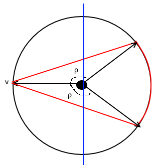
The above shows that we have a degree two pseudo-distribution \(\mu\) satisfying that with high probability over \(\{u,v\} \in E\), \(\pE_\mu (X_u-X_v)^2 \geq x_{{\mathrm{GW}}}-\e\). But we still need to show that the true maximum cut value is at most \(\alpha_{{\mathrm{GW}}}x_{{\mathrm{GW}}} + o(1)\). Luckily, here we can “stand on the shoulders of giants” and use previously known results. Specifically, by the geometric nature of this graph, intuitively the maximal cuts would be obtained via a gemoetric partition. Indeed, Borell (1975) (and, independently Sudakov and Cirel\('\)son (1974) ), proved that over the unit sphere, when we define the edge sets in such geometric terms, then the maximum cuts that optimize this will always be spherical caps. That is, the set \(S\) would be of the form \(\{ v\in \R^d : \iprod{v,a_0} \geq b_0 \}\) for some \(a_0 \in \R^d\) and \(b_0 \in \R\). Specifically, in this case, one can show that the bipartition that would maximize the number of cut edges would be a balanced one (where \(S\) and \(\cS^{d-1}\setminus S\) have the same measure) and hence \(b_0=0\). By the rotational symmetry of the sphere (and appropriately scaling \(b_0\)), we can assume without loss of generality that \(a_0\) is simply the first standard basis vector \((1,0,\ldots,0)\). Now, since a random edge \((u,v)\in E\) is chosen by letting \(v\) be a random vector with correlation roughly \(\rho_{{\mathrm{GW}}}\) with \(u\), and since the first coordinate of a random unit vector has (essentially) the Gaussian distribution with mean zero and variance \(1/n\), computing the value of the cut reduces to computing the probability that two \(\rho_{{\mathrm{GW}}}\) correlated Gaussians disagree in their sign. This latter quantity is exactly what we computed in the last lecture as \(1-\arccos(\rho_{{\mathrm{GW}}})/\pi = \alpha_{{\mathrm{GW}}}\).
Based on our construction, we can see that if the final graph has \(n\) vertices, then there is a unit vector \(v_i\) associated with each vertex \(i\), and the pseudo-expectation operator is defined as \(\pE x_ix_j = 1/2+1/2\iprod{v_i,v_j}\). The resulting matrix is the sum of the psd all-\(1/2\) matrix plus the Gram matrix (i.e., matrix of dot products) of the vectors \(\{v_1,\ldots,v_m\}\). It is not hard to verify that such a matrix is psd- see also the exercises below:
Prove that an \(n\times n\) matrix \(M\) is a psd matrix of rank \(d\) if and only if there exist \(v_1,\ldots,v_n \in \R^d\) such that \(M_{i,j}=\iprod{v_i,v_j}\).
Suppose that \(M,N\) are two \(n\times n\) psd matrices such that \(M_{i,j}=\iprod{v_i,v_j}\) and \(N_{i,j}=\iprod{u_i,u_j}\). Show explicitly a tuple of vectors \((w_1,\ldots,w_n)\) such that the psd matrix \(L=M+N\) satisfies \(L_{i,j}=\iprod{w_i,w_j}\).
Isoperimetry, extremal questions, and sum of squares
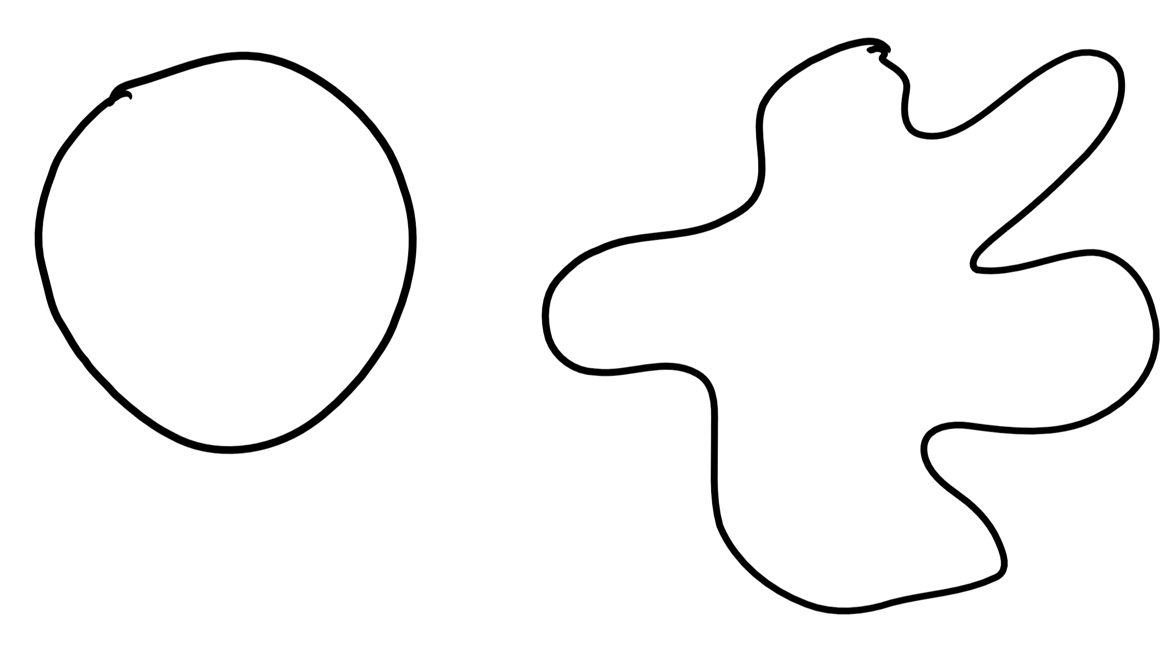
The result of (Borell 1975,Sudakov and Cirel\('\)son (1974)) we used above is one in a long line of work on isoperimetric inequalities and their many generalizations. The classical isoperimetric problem is to prove that among all shapes in the plane, the circle is the one that minimizes the ratio of its boundary to its volume. This question has been generalized to many other geometric spaces and notions of volume and boundaries. Indeed, it corresponds to the question we have already seen of finding the least expanding set in the graph: if we think of a very fine grid graph that discretizes the plane, then the isoperimetric problem corresponds to proving that the circle is the set of vertices that minimizes the expansion.
Isoperimetric questions themselves are just a special case of more general questions of finding and characterizing extremal objects. The general setting can be thought of as follows. We have:
- Some “universe” \(\cU\) of possible objects (e.g., all subsets of a graph, all closed curves in the plane, all functions or vectors in some space).
- Some “objective” function \(F:\cU\rightarrow\R\) (e.g., the ratio of boundary to volume, the sum of violations of some constraints)
- Some “nice” family \(\cS \subseteq \cU\) (e.g., shifts of circles, spherical caps, codewords)
The type of theorems we might want to prove (in increasing order of difficulty, and, often, usefulness) would be:
- An optimality theorem: If \(S\in\cU\) is a global minimum of \(F(\cdot)\) then \(S\in\cS\). Like in the isoperimetric case, such optimality theorem are often phrased as inequalities of the form \(F(S) \geq \alpha^*\) for every \(S\in\cU\), where \(\alpha^*\) is the (typically easily computable) minimum of \(F(S)\) among all the “nice” \(S\in\cS\).
- A stability theorem: If \(S\in\cU\) is a “near global minimum” (i.e., \(F(S)\) is close to \(\min_{S'\in\cU} f(S')\)) then \(S\) is “close” to some “nice” \(S^*\in\cS\). The notion of “close” here of course needs to be defined and depends on the context.
- An inverse theorem: If \(S\in\cU\) has “non trivial \(F(\cdot)\) value” (i.e., \(F(S)\) is significantly smaller than the expected value of \(F(S')\) for a random \(S'\)) then \(S\) is “somewhat correlated” with some “nice” \(S^*\in \cS\). Again, the notion of “somewhat correlated” is context-dependent. Sometimes inverse theorems come with a “list decoding” variant in which the condition is that the non-trivial value of \(F(S)\) can be explained by expressing \(S\) as some combination of a small number of “nice” objects in \(\cS\) where again what is “small” and what combinations is one allowed to take.
A related question is the notion of structure vs. randomness as discussed by Tao (see for example (Tao 2007b; Tao 2007a; Tao 2008)). Given some object \(S\in\cU\) and some family of tests/objectives \(\cF\), we want to decompose \(S\) into the “structured part” that is some combination of objects from the “nice” family \(\cS\) and the “random part” which we can think of as some “noise” object \(N\) such that \(F(N)\) is close to the expectation of \(F(S)\) over a random \(S\in\cU\) for all \(F\in\cF\).
There are often algorithmic questions associated with such theorems. One such question is the “decoding” task of finding the “nice” \(S^*\) that is close to an \(S\) with small \(F(\cdot)\) value. Another is the task of, given some description of \(\cU\) and \(F(\cdot)\), certifying an optimality theorem. Indeed, we will see that a very interesting question is often whether such an inequality has a low degree sum of squares proof. Often, an algorithmic proof of an optimality theorem will imply at least a stability theorem if not stronger results. Indeed such algorithmic proofs often give an explicit process for optimizing \(F\) that given any starting point \(S\) ends up in an optimum point. Typically, if the starting point \(S\) already had a pretty good \(F(\cdot)\) value then the algorithm would presumably not take too many steps and hence its final output will be “close” to the initial point.
At this point, when we’ve seen only one concrete example, this discussion might feel somewhat abstract, but many important results, including hypercontractivity, the “invariance principle”, Brascamb Lieb inequalities, results on list decoding, the Gowers norm, and others can be thought of as falling into this general framework. We will see several other examples of such results in this course.
Beyond degree \(2\)
The examples above show that the rounding algorithms of the previous lecture are tight with respect to degree two pseudodistributions. But of course, we can run the sum of squares algorithm for larger degrees. We do pay a price in the running time, but it remains polynomial time for every constant degree, and as long as the degree is significantly smaller than \(n\) it would still be significantly faster than brute force.
Could it be that using larger, but still small degree, we can beat the guarantees for max cut, graph expansion, or boolean quadratic forms that are achieved respectively by Goemans-Willamson, Cheeger, or Grothendieck? The short answer that we do not know. It is known that if Khot’s Unique Games Conjecture is true (or the closely related Small Set Expansion Hypothesis) then no polynomial (or even \(2^{n^{o(1)}}\) time) algorithms can beat those guarantees. In particular, for every \(d = n^{o(1)}\) these conjectures predict that we can obtain instances with the same gaps as we showed in this lecture but with respect not to merely degree \(2\) but to the value achieved by degree \(d\) pseudo-distributions. However, even for \(d=O(1)\) (even \(d=4\)) this is still wide open. What we do know is that the same examples that we saw in this leture do not yield such gaps. Here is one example:
Let \(n\) be odd and \(C_n\) be the \(n\)-length cycle. Prove that for every degree \(6\) pseudo-distribution \(\mu\) over \(\bits^n\), \(\pE_\mu f_{C_n} \leq (1-1/n)|E|\).Hint: Start by showing the square triangle inequality for degree \(6\) pseudo-distributions. That is prove that for every degree \(6\) pseudo-distribution \(\mu\) over \(\bits^n\) and every \(i,j,k\in [n]\), \(\pE_\mu (x_i-x_k)^2 \leq \pE_\mu (x_i-x_j)^2+(x_j-x_k)^2\).
References
Borell, Christer. 1975. “The Brunn-Minkowski Inequality in Gauss Space.” Invent. Math. 30 (2): 207–16.
Feige, Uriel, and Gideon Schechtman. 2002. “On the Optimality of the Random Hyperplane Rounding Technique for MAX CUT.” Random Struct. Algorithms 20 (3): 403–40.
O’Donnell, Ryan. 2014. Analysis of Boolean Functions. Cambridge University Press, New York. doi:10.1017/CBO9781139814782.
Sudakov, V. N., and B. S. Cirel\('\)son. 1974. “Extremal Properties of Half-Spaces for Spherically Invariant Measures.” Zap. Naučn. Sem. Leningrad. Otdel. Mat. Inst. Steklov. (LOMI) 41: 14–24, 165.
Tao, Terence. 2007a. “Structure and Randomness in Combinatorics.” In FOCS, 3–15. IEEE Computer Society.
———. 2007b. “The Dichotomy Between Structure and Randomness, Arithmetic Progressions, and the Primes.” In International Congress of Mathematicians. Vol. I, 581–608. Eur. Math. Soc., Zürich. doi:10.4171/022-1/22.
———. 2008. Structure and Randomness. American Mathematical Society, Providence, RI. doi:10.1090/mbk/059.